
| 일 | 월 | 화 | 수 | 목 | 금 | 토 |
|---|---|---|---|---|---|---|
| 1 | 2 | 3 | 4 | |||
| 5 | 6 | 7 | 8 | 9 | 10 | 11 |
| 12 | 13 | 14 | 15 | 16 | 17 | 18 |
| 19 | 20 | 21 | 22 | 23 | 24 | 25 |
| 26 | 27 | 28 | 29 | 30 | 31 |
- 데이터 증식
- 인프런
- 3기가 마지막이라니..!
- 데이터 정합성
- WITH ROLLUP
- splitlines
- 컨브넷
- DENSE_RANK()
- python
- ImageDateGenerator
- 리프 중심 트리 분할
- 부트 스트래핑
- 캐글 신용카드 사기 검출
- 그룹 연산
- Growth hacking
- 스태킹 앙상블
- 그로스 해킹
- WITH CUBE
- lightgbm
- 로그 변환
- XGBoost
- sql
- 데이터 핸들링
- 캐글 산탄데르 고객 만족 예측
- 분석 패널
- 그로스 마케팅
- tableau
- 마케팅 보다는 취준 강연 같다(?)
- pmdarima
- ARIMA
- Today
- Total
LITTLE BY LITTLE
[ch_03] Hands on Data Analysis With Pandas - Data Wrangling (reindex, pivoting, unstack, melt, clip, ffill, interpolate ..) 본문
[ch_03] Hands on Data Analysis With Pandas - Data Wrangling (reindex, pivoting, unstack, melt, clip, ffill, interpolate ..)
위나 2022. 10. 6. 19:21ch_03.
- wide_vs_long
- wide가 일반적으로 많이 본 형태, describe로 한 눈에 볼때 편리, pandas의 matplotlib로 시각화
- long은 컬럼명이 data type과 value로 구성, describe하기에 적절치 않음, seaborn으로 시각화
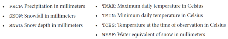
- using_the_weather_api
- cleaning_data
- df.rename(str.supper(axis='columns').columns
- pd.to_datetime(df.col)
- pd.tz_localize(), pd.tz_convert(), pd.tz_localize(None).to_period('M').to_timestamp().index
- assign()으로 한번에 데이터 타입 변경 (df.col.astype('int' or ..))
- 범주형으로 변경 col = df.col.astpe('category')
- 카테고리 생성 pd.Categorical(['a','b','a','a','c','c'], categories=['A','B','C'],ordered=True)
- 범주형의 describe만 출력 df_with_categories.descrbie(include='category')
- df[df.datatype == 'TMAX'].sort_values(by='temp_C', ascending=False) 정렬
- 중복된 값의 경우 date 순서대로 정렬되지 않아서, date도 같이 정렬해주는 것이 좋다.
- df[df.datatype == 'TMAX'.sort_values(by=['temp_C','date'],ascending=[False,True]).head()
- df.sort_values(ignore_index=True) 할경우 정렬된 데이터프레임에 인덱스 새로 설정
- df.sort_index(axis=1).head().loc[:,'temp_C':'temp_F_whole'] loc 더 쉽게 가능
- .nlargest(), .nsmallest(), .sample()
- datetime은 슬라이싱할 때 처음과 끝 모두 포함(원래 끝 값은 제외)
- reset_index : 데이터를 잃고싶지 않을 때 사용
- date에서 day of week 컬럼 생성 => assign(day_of_week=lambda x: x.index.day_name())
- 인덱스가 달라지는 문제
- reindex가 필요 => reindex(df.index).head().assign(day_of_week=lambda x:x.index.day_name())
- reindex 옵션으로 Nan 채우기 - df.reindex(df.index,method='ffill')
- df.col.fillna(0) / df.col.fillna(method='ffill')
- reshaping_data
- long은 데이터들이 행(->)방향으로 나열, wide는 열 방향(아래)으로 나열
- pivoting : index, columns, values 세가지를 지정해서 자유롭게 데이터프레임을 만들어서 볼 수 있다.
- 특정 컬럼 순서로 보고싶을 때 pivoted_df['temp_F']['TMIN']
- 인덱스 여러개(멀티 인덱스) 설정 가능 df.set_index(['col1','col2'])
- 멀티 인덱스 해제 unstakced_df = multi_index_df.unstack()
- unstack에도 결측치 채우는 옵션 - df.unstack(fill_value=0)
- 결측치를 어떻게 채울지 보고싶을 때 unstack()을 많이 사용
- 데이터 추가 df.append([{..}]) <= 리스트 안에 딕셔너리 형태로
- melt : 컬럼을 녹여서 행으로 보냄
- wide_df.melt(id_vars='date', value_vars= ['col1','col2','col3'],value_name = 'value', var_name = 'col')
- pivoting 대신에 date를 인덱스로 설정하고, stack() 한 후에 stacked_series.to_frame('values') 데이터프레임으로 바꾸면 melted됨
- handling_data_issues
- df.duplicated(keep=False)로 설정하면 중복된 여러개 값 중 첫번째는 중복에서 제외, 유지함
- col.combine_first(another_col) => 다른 객체로 결측치를 덮어 쓸 수 있다
- df.col.dropna(axis='column', how='all',subset=['col1','col2'],thresh=df.shape[0]*.75)
- how=all일경우 해당 열의 데이터가 전체다 null이어야만 삭제됨
- * thresh는 shape[0],즉 열의 개수 기준 데이터가 75%개 미만으로 입력되었을시 drop하는 옵션
- 매일 급격히 변하지않는 데이터의 경우, 바로 앞/뒤 값으로 결측치를 채우는 ffill, bfill이 적합한 방법
- NaN은 0으로, inf/-inf는 유한한 값으로 바꿔주는 np.nan_to_num(col)
- clip(lower bound, col) => clip도 np.nan_to_num과 같은 기능이지만, 최대/최대 threshold를 정할 수 있음 (ex. 음수가 될 수 없는 컬럼의 값의 lower bound를 0으로 정할 수 있다)
- fillna(x,rolling(7,min_periods=0).median() => 이동 중앙값으로 결측치를 채울 수 있다
- min_periods=0으로 설정하면 기간이 아무리 적어도 결괏값을 얻을 수 있음
- x.interpolate() 선형으로 결측치를 채우는 방법
3-1. wide VS long
wide

=> wide가 일반적으로 봐왔던 형태
import matplotlib.pyplot as plt
import pandas as pd

wide_df = pd.read_csv('data/wide_data.csv', parse_dates=['date'])
long_df = pd.read_csv(
    'data/long_data.csv',
    usecols=['date', 'datatype', 'value'],
    parse_dates=['date']
)[['date', 'datatype', 'value']] # sort columns
Wide(↓)는 describe로 한 눈에 볼 때 편리함
wide_df.describe(include='all', datetime_is_numeric=True)wide_df.plot(
x='date', y=['TMAX', 'TMIN', 'TOBS'], figsize=(15, 5),
title='Temperature in NYC in October 2018'
).set_ylabel('Temperature in Celsius')
plt.show()
Long

=> long은 컬럼명이 데이터 속에 들어가있고, data type, value로(↓) 나열
=> long은 describe하기에 적절치 않음
=> plot으로 그릴때에도 pandas가 아닌 seaborn 이용하는 것이 더 적합
import seaborn as sns

sns.set(rc={'figure.figsize': (15, 5)}, style='white')

ax = sns.lineplot(
    data=long_df, x='date', y='value', hue='datatype'
)
ax.set_ylabel('Temperature in Celsius')
ax.set_title('Temperature in NYC in October 2018')
plt.show()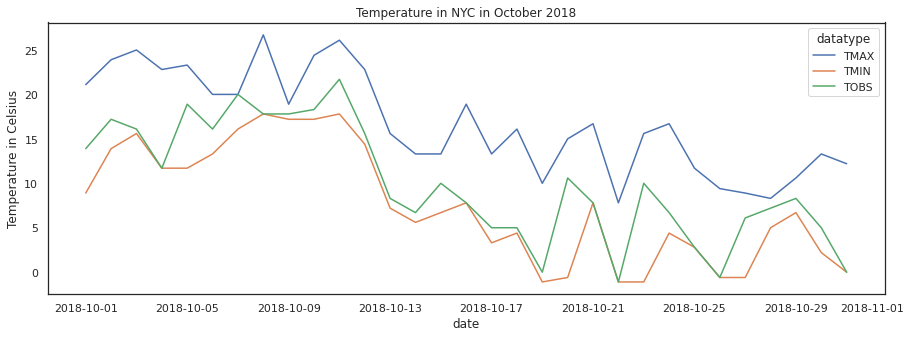
long data와 seaborn으로 facet plots
sns.set(
    rc={'figure.figsize': (20, 10)}, style='white', font_scale=2
)

g = sns.FacetGrid(long_df, col='datatype', height=10)
g = g.map(plt.plot, 'date', 'value')
g.set_titles(size=25)
g.set_xticklabels(rotation=45)
plt.show()
3-2. Using the weather api
central_park 여기서 .,,
3-3. Cleaning Data

import pandas as pd

df = pd.read_csv('/content/nyc_temperatures.csv')
df.head()
.rename()
df.rename(
    columns={
        'value': 'temp_C',
        'attributes': 'flags'
    }, inplace=True
)
rename + string operations
df.rename(str.upper, axis='columns').columnspd.to_datetime()
df.loc[:,'date'] = pd.to_datetime(df.date)
df.dtypespd.tz_localize()
pd.tz_convert()
period monthly로 변경
eastern.tz_localize(None).to_period('M').index.to_timestamp()
eastern.tz_localize(None).to_period('M').to_timestamp().index.assign()으로 한번에 데이터 타입 변경
new_df = df.assign(
    date=pd.to_datetime(df.date),
    temp_F=(df.temp_C * 9/5) + 32
)
assign()은 주로 lambda식과 함께 씀, astype() 사용
df = df.assign(
    date=lambda x: pd.to_datetime(x.date),
    temp_C_whole=lambda x: x.temp_C.astype('int'),
    temp_F=lambda x: (x.temp_C * 9/5) + 32,
    temp_F_whole=lambda x: x.temp_F.astype('int')
)
카테고리 생성, astype('category')
df_with_categories = df.assign(
    station=df.station.astype('category'),
    datatype=df.datatype.astype('category')
)
df_with_categories.dtypes
카테고리 정렬
pd.Categorical(
    ['med', 'med', 'low', 'high'],
    categories=['low', 'med', 'high'],
    ordered=True
)
df_with_categories.describe(include='category')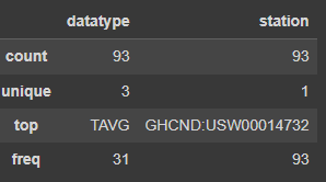
df['정렬대상 컬럼'].sort_values(by='정렬기준 컬럼')
df[df.datatype == 'TMAX'].sort_values(by='temp_C', ascending=False).head(10)이렇게 할시, temp_C가 같은 값일 경우, date가 뒤죽박죽되어 출력, date도 정렬해주기
df[df.datatype == 'TMAX'].sort_values(by=['temp_C', 'date'], ascending=[False, True]).head(10)sort_values(ignore_index=True) 정렬된 데이터프레임에 인덱스 새로 설정
df[df.datatype == 'TMAX'].sort_values(by=['temp_C', 'date'], ascending=[False, True], ignore_index=True).head(10).nlargest
df[df.datatype == 'TAVG'].nlargest(n=10, columns='temp_C').nsmallest
df.nsmallest(n=5, columns=['temp_C', 'date'])df.sample(5, random_state=0).index.sort_index() 인덱스도 정렬가능
df.sort_index(axis=1).head().sort_index()이용해서 loc 더 쉽게 할 수 있다
df.sort_index(axis=1).head().loc[:,'temp_C':'temp_F_whole']* 같은 데이터이더라도, 인덱스가 다르면 not-equal 출력 (ex. sort_values한 df와 그냥 df는 다름)
=> 하지만 sort_values한 data frame도 sort_index하면 같아짐
2018년 출력
df.loc['2018']2018년 4분기 출력
df.loc['2018-Q4']datetime은 slicing할 때 inclusive of both endpoints
df['2018-10-11':'2018-10-12'](*.reset_index()는 데이터를 잃고싶지 않을 때 (인덱스로 설정한 컬럼의 데이터) 자주 사용된다.)
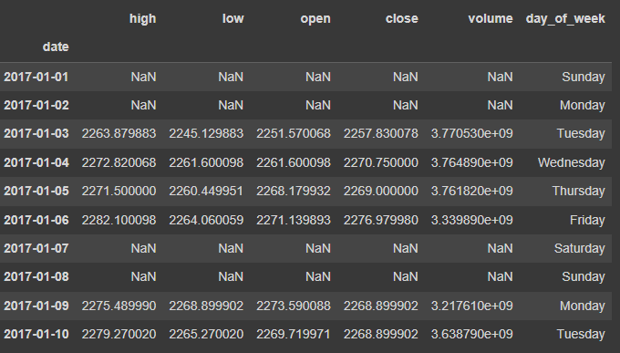
index_col을 date로 설정해서 불러온 뒤, index인 date의 day를 호출해서 day_of_week 컬럼 추가로 생성
(컬럼 추가 생성으로 인해 인덱스가 달라지는 문제가 생김)
sp = pd.read_csv(
    '/content/sp500.csv', index_col='date', parse_dates=True
).drop(columns=['adj_close'])

sp.head(10).assign(
    day_of_week=lambda x: x.index.day_name()
)
근데 위의 경우 문제가 있다. reindex가 필요, 문제를 그래프로 그려서 확인
import matplotlib.pyplot as plt # we use this module for plotting
from matplotlib.ticker import StrMethodFormatter # for formatting the axis

# plot the closing price from Q4 2017 through Q2 2018
ax = portfolio['2017-Q4':'2018-Q2'].plot(
    y='close', figsize=(15, 5), legend=False,
    title='Bitcoin + S&P 500 value without accounting for different indices'
)

# formatting
ax.set_ylabel('price')
ax.yaxis.set_major_formatter(StrMethodFormatter('${x:,.0f}'))
for spine in ['top', 'right']:
    ax.spines[spine].set_visible(False)

# show the plot
plt.show()
align the index by using reindex() method
sp.reindex(bitcoin.index).head(10).assign(
    day_of_week=lambda x: x.index.day_name()
)
reindex 전
reindex 후
주말과 공휴일의 값이 NaN인 것을 forward-fill로 채워서 해결하자, reindex(index, method='ffill')
sp.reindex(bitcoin.index, method='ffill').head(10)\
.assign(day_of_week=lambda x: x.index.day_name())reindex(index).compare() method로 ffill이 잘 되었는지 확인
#To isolate the changes happening with the forward-filling, we can use the `compare()` method.

sp.reindex(bitcoin.index)\
    .compare(sp.reindex(bitcoin.index, method='ffill'))\
    .head(10).assign(day_of_week=lambda x: x.index.day_name())
self가 forward-fill 이전, other가 forward-fill 이후
=> 주말과 공휴일이 forward-filled로 채워진 값을 갖고있음을 알 수 있다.
추가로 0으로 결측치를 채워넣자
import numpy as np

sp_reindexed = sp.reindex(bitcoin.index).assign(
    volume=lambda x: x.volume.fillna(0), # put 0 when market is closed
    close=lambda x: x.close.fillna(method='ffill'), # carry this forward
    # take the closing price if these aren't available
    open=lambda x: np.where(x.open.isnull(), x.close, x.open),
    high=lambda x: np.where(x.high.isnull(), x.close, x.high),
    low=lambda x: np.where(x.low.isnull(), x.close, x.low)
)
sp_reindexed.head(10).assign(
    day_of_week=lambda x: x.index.day_name()
)
시각화해서 reindexing이 어떻게 market이 closed되었을 때의 asset value가 유지될 수 있게 해주었는지 확인
# every day's closing price = S&P 500 close adjusted for market closure + Bitcoin close (same for other metrics)
fixed_portfolio = sp_reindexed + bitcoin

# plot the reindexed portfolio's closing price from Q4 2017 through Q2 2018
ax = fixed_portfolio['2017-Q4':'2018-Q2'].plot(
    y='close', label='reindexed portfolio of S&P 500 + Bitcoin', figsize=(15, 5), linewidth=2,
    title='Reindexed portfolio vs. portfolio with mismatched indices'
)

# add line for original portfolio for comparison
portfolio['2017-Q4':'2018-Q2'].plot(
    y='close', ax=ax, linestyle='--', label='portfolio of S&P 500 + Bitcoin w/o reindexing'
)

# formatting
ax.set_ylabel('price')
ax.yaxis.set_major_formatter(StrMethodFormatter('${x:,.0f}'))
for spine in ['top', 'right']:
    ax.spines[spine].set_visible(False)

# show the plot
plt.show()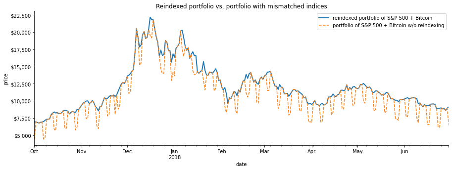
3-4. Reshaping data
( wide ↓ / long → 에 따라 데이터 형식 바꿀 필요가 있음 )
- Pivoting
- unstack
- melt
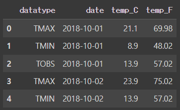
long_df = pd.read_csv('data/long_data.csv',usecols = ['date','datatype','value']).rename(
columns={'value':'temp_C'}).assign(date=lambda x: pd.to_datetime(x.date),
temp_F = lambda x: (x.temp_C * 9/5) + 32)
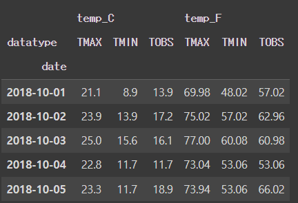
long_df.head()wide_df = pd.read_csv('data/wide_data.csv')
wide_df.head()[Out]

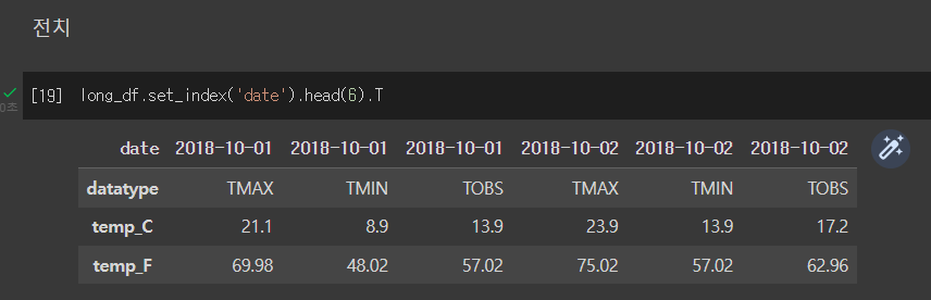
Transpose
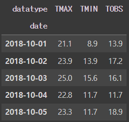
Pivoting - 특정 컬럼을 인덱스로 쓸 때 (ex. 날짜 컬럼 기준으로 long format data 나열)
- index, columns, values 다 설정할 수 있다.
pivoted_df = long_df.pivot(
    index = 'date', columns='datatype', values = 'temp_C'
)
pivoted_df.head()
[Out]
values 여러개 설정
pivoted_df = long_df.pivot(index='date', columns='datatype',
                           values=['temp_C','temp_F'])
pivoted_df.head()
[Out]

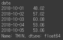
특정 컬럼 순서로 보고싶을 때
pivoted_df['temp_F']['TMIN'].head()[Out]
인덱스를 여러개 설정하고 싶을 때 set.index([리스트])
multi_index_df = long_df.set_index(['date','datatype'])
multi_index_df.head().index
multi_index_df.head()
[Out]
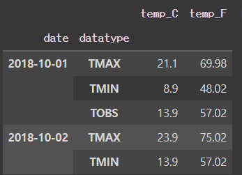
멀티 인덱스 해제 - unstack(<->pivoted)
unstacked_df = multi_index_df.unstack()
unstacked_df.head()
[Out]
unstack()은 결측치 채울 때 어떻게 채워야할지 보고자 하는데 도움을 준다
결측치를 임의로 만들기위해서 append로 데이터 추가해주기
extra_data = long_df.append([{
    'datatype' : 'TAVG',
    'date' : '2018-10-01',
    'temp_C' : 10,
    'temp_F' : 50
}]).set_index(['date','datatype']).sort_index()

extra_data['2018-10-01':'2018-10-02']
[Out]

extra_data.unstack().head()[Out]

unstack(fill_values) 옵션으로 결측치 채우기
extra_data.unstack(fill_value=-40).head()[Out]

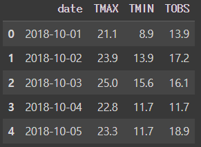
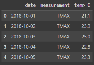
MELT : 컬럼을 녹여서 행으로 보냄
melted_df = wide_df.melt(id_vars = 'date', value_vars = ['TMAX', 'TMIN', 'TOBS'],
                         value_name = 'temp_C', var_name = 'measurement')
melted_df.head()
[Out] (오른쪽)
Pivoting(인덱스 설정)하는 다른 방법은 1) stack()하고, 2) stack() 메소드로 melt 시키는 방법
1) stack() 하기
wide_df.set_index('date', inplace=True)
stacked_series = wide_df.stack() # 인덱스에 데이터타입 넣기
stacked_series.head()
[Out]
2) melt 시키기(컬럼을 녹여서 행으로) : to_frame으로 values 지정
stacked_df = stacked_series.to_frame('values')
stacked_df.head()
[Out] (왼쪽)


3-5. Handling Data Issues
df.describe()[Out]

df.info()[Out]
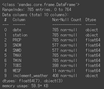
컬럼별로 isna()를 데이터 프레임으로 만들어서 shape[0] 확인 => 결측치 총 개수는 765개
contain_nulls = df[
    df.SNOW.isna() | df.SNWD.isna() | df.TOBS.isna()
    | df.WESF.isna() | df.inclement_weather.isna()
]
contain_nulls.shape[0]
# 765contain_nulls.head(10)[Out]

import numpy as np
df[df.inclement_weather == 'NaN'].shape[0] # doesn't work
df[df.inclement_weather == np.nan].shape[0] # doesn't work
isna()써야 shape 확인 가능
df[df.inclement_weather.isna()].shape[0]isin()
df[df.SNWD.isin([-np.inf])].shape[0]na는(np.inf ~ -np.inf) 사이 값이 아니라서, 이런식으로 찾을경우 없다고 나옴
def get_inf_count(df):
  return {
      col: df[
          df[col].isin([np.inf, -np.inf])
      ].shape[0] for col in df.columns
  }
get_inf_count(df)
[Out]
{'date': 0,
 'station': 0,
 'PRCP': 0,
 'SNOW': 0,
 'SNWD': 577,
 'TMAX': 0,
 'TMIN': 0,
 'TOBS': 0,
 'WESF': 0,
 'inclement_weather': 0}
inf
snow depth 컬럼에 inf 값 존재 여부 확인
pd.DataFrame({
    'np.inf Snow Depth': df[df.SNWD == np.inf].SNOW.describe(),
    '-np.inf Snow Depth': df[df.SNWD == -np.inf].SNOW.describe()
}).T
[Out]

중복
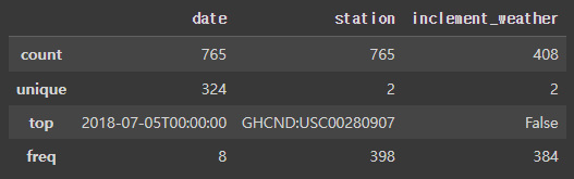
범주형 변수만 describe로 개수 unique(=null이 아닌 값) 개수 확인
df.describe(include='object')[Out]
duplicated()로 중복 값이 있는 row 찾기
df[df.duplicated()].shape[0]

df[df.duplicated(keep=False)].shape[0]

df[df.duplicated()].head()
=> 디폴트인 keep=True로 하면 중복된 값의 첫번째는 중복으로 치지 않음 => 284
=> keep=False로해서 첫번째 값도 중복으로 처리 => 284
=> 특정 컬럼의 중복값만 확인 가능
=> Let's look at a few duplicates. Just in the few values we see here, we know that the top 4 are actually in the data 6 times because by default we aren't seeing their first occurrence: ?????
# 1. 날짜 컬럼 datetime으로 형식 변경
df.date = pd.to_datetime(df.date)

# 2. save this information for later
station_qm_wesf = df[df.station == '?'].drop_duplicates('date').set_index('date').WESF

# 3. 값이 ?인 부분을 아래로 오게 정렬(내림차순)
df.sort_values('station', ascending=False, inplace=True)

# 4. keep=True로 설정해서 중복 값의 첫번째만 유지
# 값이 있을 시 valid한 station이 되도록
df_deduped = df.drop_duplicates('date')

# 5. 중복값 처리하기 이전 원본 컬럼 삭제
df_deduped = df_deduped.drop(columns='station').set_index('date').sort_index()

# 6. take valid station's WESF and fall back on station ? if it is null
df_deduped = df_deduped.assign(
    WESF=lambda x: x.WESF.combine_first(station_qm_wesf)
)

df_deduped.shape
=> 마지막에 combine_first() 메소드로 다른 객체로 결측치 덮어씀
=> 즉, valid한 WESF값을 갖고있는 데이터의 station 값을 결측치가 있는 데이터에 덮어 쓰는 것

결측치
df_deduped = df[df.duplicated()]

df_deduped.dropna().shape

df_deduped.dropna(how='all').shape # 디폴트는 how='any'

df_deduped.dropna(
    how='all', subset=['inclement_weather', 'SNOW', 'SNWD']).shape

df_deduped.dropna(
    axis='columns',
    thresh = df_deduped.shape[0] * .75 # 열의 75%라는 의미
).columns
=> dropna에서 how='all'으로 지정할경우, 값이 "전부 다" null인 경우에만 삭제하기 때문에, 아무것도 삭제되지 않음, shape이 원본과 같이 (324,8)
=> dropna에 subset=리스트로 특정 컬럼의 결측치만 drop
=> threshold를 정해서 컬럼을 기준으로 값이 n개 미만 입력되었을시 컬럼을 drop => drop thresh = df_deduped.shape[0] * .75 => 데이터의 shape 에서 데이터 수를 가져온 후 75% 값보다 적게 있으면 drop!
[Out]
Index(['date', 'station', 'PRCP', 'SNOW', 'SNWD', 'TMAX', 'TMIN'], dtype='object')loc으로 특정 컬럼 선택해서 그 컬럼의 null을 fillna로 채우기
df_deduped.loc[:, 'WESF'].fillna(0, inplace=True)
df_deduped.head()
Unreasonable values
필수는 아니지만 경우에 따라 필요한 작업
temperature 데이터에서
1. TMAX (=temperature of the Sun) 에는 measured_value가 없어야하므로, 5505 => NaN으로 대체
2. TMIN 은 -40°C를 placeholder로 사용하고 있지만, NYC에서 가장 추운 날의 기온은 -26.1°C이기 때문에 -40°C=>NaN
df_deduped = df_deduped.assign(
    TMAX = lambda x: x.TMAX.replace(5505, np.nan),
    TMIN = lambda x: x.TMIN.replace(-40, np.nan)
)
df_deduped.assign(
TMAX = lambda x: x.TMAX.fillna(method='ffill'),
TMIN = lambda x: x.TMIN.fillna(method='ffill')
).head()Unreasonable values => NaN으로 바꾼 뒤, 기온은 매일 급격히 변하지는 않기 때문에, 결측치를 바로 앞/뒤 기온으로 채워넣어주는 방법도 적합 (ffill/bfill)
df_deduped.assign(
    TMAX=lambda x: x.TMAX.fillna(method='ffill'),
    TMIN=lambda x: x.TMIN.fillna(method='ffill')
).head()
NaN와 inf 값을 np.nan_to_num() 함수로 처리
- NaN => 0
- inf/-inf는 => 아주 큰 유한한 값이 됨
df_deduped.assign(
    SNWD=lambda x: np.nan_to_num(x.SNWD)
).head()
[Out]

Clip() 메소드도 np.nan_to_num()과 같은 기능, 차이점은 특정 최소/최대 threshold를 정할 수 있다.
=> SNWD 컬럼은 음수가 될 수 없기 때문에, clip()으로 lower bound를 0으로 정하자
df_deduped.assign(
    SNWD=lambda x: x.SNWD.clip(0, x.SNOW)
).head()
[Out]

TMAX와 TMIN의 결측치를 median으로, TOBS의 결측치를 TMAX와 TMIN의 평균으로 정해주자
(assign + lambda 함수사용)
df_deduped.assign(
    TMAX=lambda x: x.TMAX.fillna(x.TMAX.median()),
    TMIN=lambda x: x.TMIN.fillna(x.TMIN.median()),
    # average of TMAX and TMIN
    TOBS=lambda x: x.TOBS.fillna((x.TMAX + x.TMIN) / 2)
).head()
[Out]

apply()를 이용해서 컬럼 사이 같은 연산을 적용
rolling 7-day median 이동 중앙값 으로 결측치를 채워넣자. => ch4.에서 rolling calculations 다룸
df_deduped.apply(
    # rolling calculations will be covered in chapter 4, this is a rolling 7-day median
    # we set min_periods (# of periods required for calculation) to 0 so we always get a result
    lambda x: x.fillna(x.rolling(7, min_periods=0).median())
).head(10)
마지막은 interpolate() 으로 결측치 채우는 방법
디폴트는 linear
1월 9일 데이터가 없기 때문에, 8일과 10일의 평균값으로 (=interpolate) 결측치 채우기
df_deduped\
    .reindex(pd.date_range('2018-01-01', '2018-12-31', freq='D'))\
    .apply(lambda x: x.interpolate())\
    .head(10)


